As stated in a previous post, tuning PID controllers is a multi-step process. After you gather your data from your step test, the next step in the process is fitting a model to your Process Data. Fitting a model involves the analysis of bump test data and the calculation of tuning parameters that are specific to both your controller and your control objective. This post highlights some industry best practices for fitting a model to your test data.
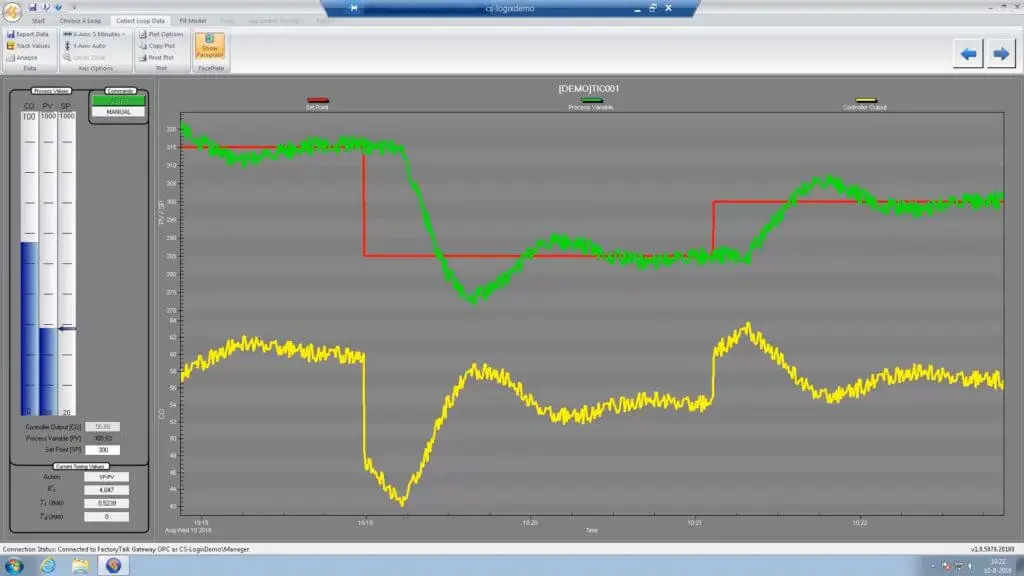
Before you can even start to model your data, you need to have caused a clear change. This can be done by performing a step test. If you need to brush up on how to perform a step test, you can read our previous post here.
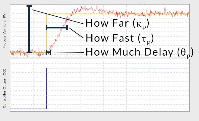
A good model should accurately describes three (3) things: How Far, How Fast, and How Much Delay. The how far variable, also known as Process Gain, describes how far the Process Variable will travel in response to a given change in Controller Output. The how fast variable is also known as the Process Time Constant. This variable describes how quickly the Process Variable moves in response to a change in the Controller Output. Finally, there is the Process Dead-Time which is the variable that represents how much delay exists in a process. More specifically Dead-Time is the delay from when a change in Controller Output is first initiated until the time that the measured Process Variable first begins to respond. The presence of Dead-Time is never a good thing in a control loop. While different processes have varying amounts of Dead-Time, when Dead-Time becomes equal or greater to your Process Time Constant, it can wreak havoc on your control objectives. Once you can understand these elements of your process data you are ready to create your model.

When modeling, it is best to have data at opposite extremes of the process. The picture above shows the bump tests performed for a temperature application. The red bars cover the area where the process is “heating up” while the blue bar represents where the process is “cooling down”. Having data from both these events will allow you to see if there is a change in dynamics in one direction or another. When creating your model, capture several model segments around these “heating” and “cooling” sections so that you are able to compare and contrast. While the example of “heating” and “cooling” were used above, the thing to keep in mind it to capture models from opposite spectrums. If this example were changed to a valve, you would want to gather data from when the valve opened and when it closed.
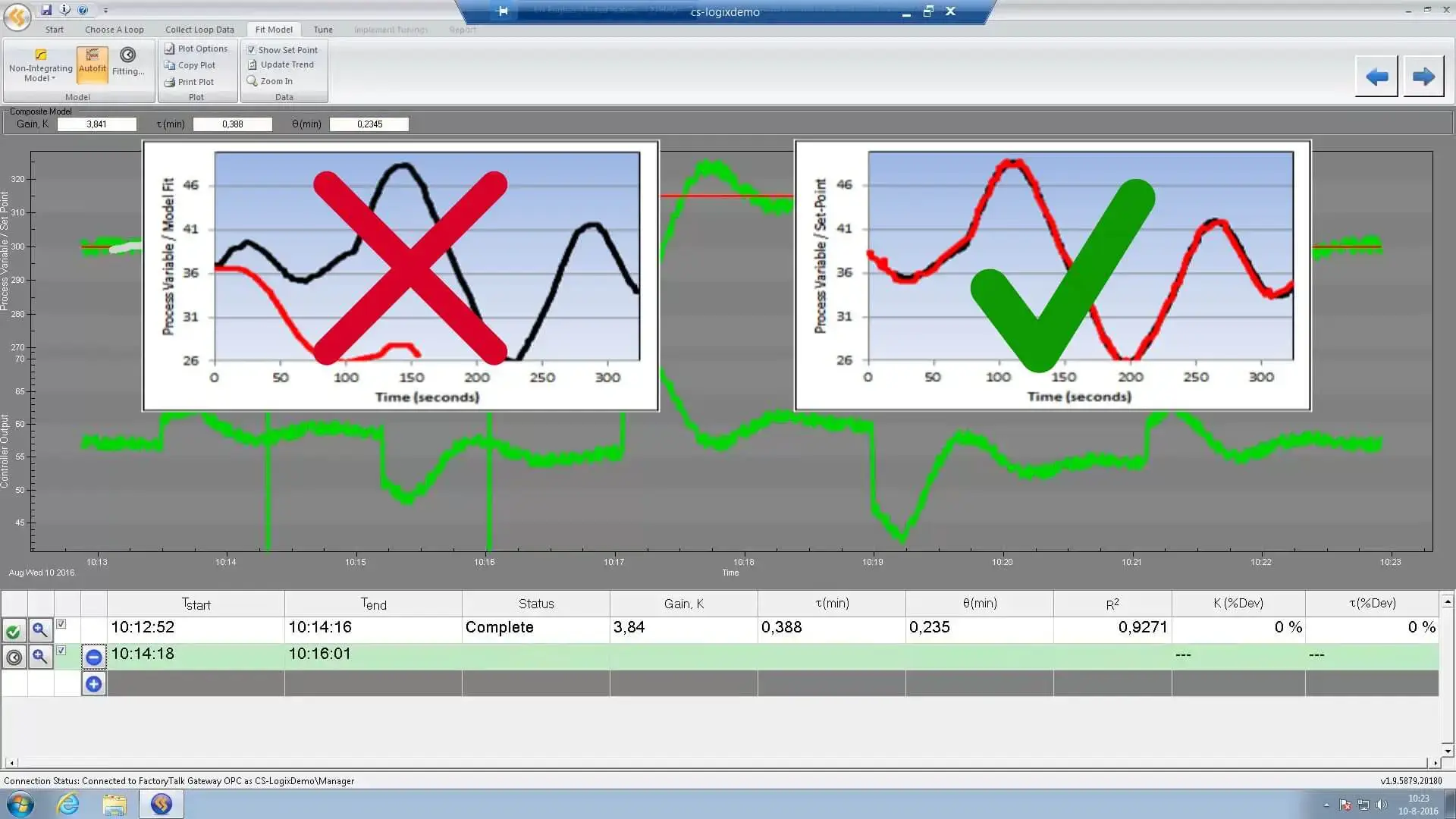
A question that we see a lot is: “What constitutes a good model?”. The best way to determine a good model is looking at how accurately the model describes the underlying data. In the picture above, there are two models shown, one poorly fitted model and one well fitted model. The model on the left, which is illustrated by a red line, doesn’t track anywhere close to the black line which represents the Process Data. It is safe to say that this is not a good model. The model on the right on the other hand is an example of a good model. Notice that the model closely follows the Process Data. Even though it seems simple enough, it is surprising how often not properly fitting a model can throw a wrench into the tuning process.
While many in the industry use software that allows for visual modeling, what do you do if you need to model manually? The most common way to model manually is by using the First Order Plus Dead -Time or FOPDT modeling. There are three (3) steps in this process. First, you must calculate the Process Gain.
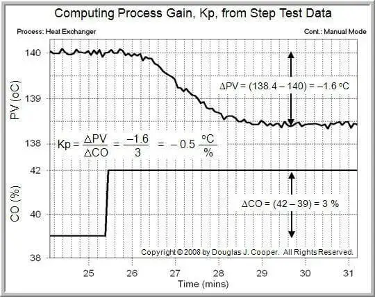
This graphic demonstrates how to calculate the Process Gain. For more details, visit Control Guru. Next, you will need to calculate the Process Time Constant.
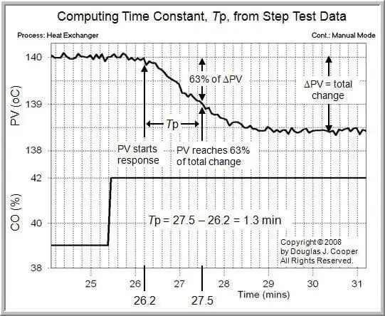
This graphic demonstrates how to calculate the Process Time Constant. For more details, visit Control Guru. Finally, you will need to find the amount of Dead-Time.
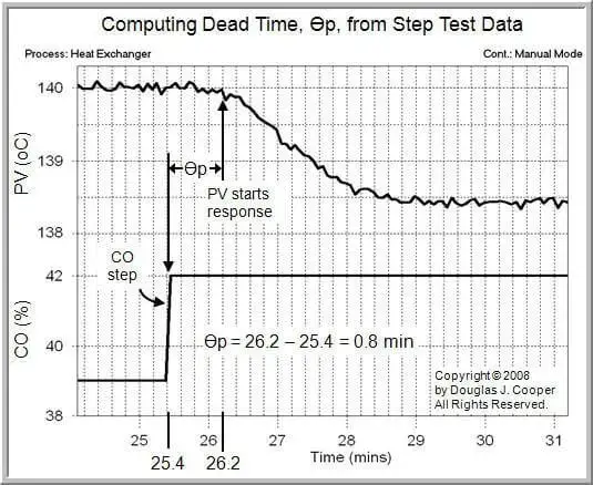
This graphic demonstrates how to calculate the Dead-Time. For more details, visit Control Guru. When you calculate the values for the Process Gain, Process Time Constant, and Dead-Time, you are ready to move on to the tuning stage.
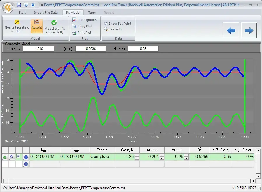
One final thing you need to consider is software. As seen above, modeling can be done by hand. However, software provides more accurate and consistent results. Furthermore, you need software that is equipped to handle the oscillatory and noisy data that is often found in the “real-world”. The image above shows a model of highly dynamic, “real-world” data that was calculated with the help of software. Be forewarned, not all software is equipped with the ability to model data that is noisy and oscillatory. If you do decide to look for PID optimization software, be sure to look for software that can handle data at a Non-Steady State.
If you need additional guidance on how to perform a test or how to tune your PIDs for optimal performance, consider attending a training workshop that focuses on understanding process dynamics and the PID controller or contact us.


